
Ques 2(a). An iron ring has a cross-sectional area of 200 mm2 and a mean diameter of 20 cm. It is wound with 1000 turns. If the value of relative permeability is 250. Find the total flux set up in the ring. The coil resistance is 500 Ω and the supply voltage is 220V
Ans(a). The figure of the above question is given below
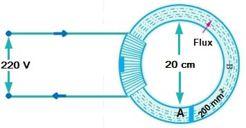
Given
Area = 200 mm2
Number of turns N = 1000 turns
Resistance R = 500Ω
Voltage V = 220 V
Relative permeability μr = 250
The field strength inside the solenoid is
[latex display=”true”]H = \dfrac{{NI}}{l}{\text{ AT/m}}[/latex]
Where N = Number of turns
I = current
l = length
Now I = V/R = 220/500 = 0.44 A
l = πD = π × (20 × 10-2) = 0.628 m
[latex display=”true”]\begin{array}{l}H = \dfrac{{1000 \times 0.44}}{{0.628}}{\rm{ }}\\\\{\text{ = 700 AT/m}}\end{array}[/latex]
Now magnetic flux density B
B = μoμrH
Where
H = magnetic field strength,
µo = permeability of free space
μr = relative permeability of the core respectively.
= 4π × 10-7 × 250 × 700
B = 219.91 × 10⁻³ T
Hence Total Flux in the coil Φ
Φ = B × A
= 219.91 × 10-3 × 200 × 10-6
= 43.982 × 10⁻⁶ Wb.
Ques 2(b). Define the following terms:
(i) Coefficient of magnetic coupling
(ii) Self-Inductance
(iii) Electromagnetic Induction
(iv) Time constant
Ans.
Coefficient of Magnetic Coupling
During Mutual Inductance between two coils, we assume that the flux produced by one coil is entirely linked with the other coil. But practically it is not true, the certain portion of the flux of one coil does not link with the other coil.
The ratio of the portion of the flux of one coil link with the other coil to the entire flux produced by the coil is referred as the coefficient of magnetic coupling.
or
The coupling coefficient K is the degree or fraction of magnetic coupling that occurs between the circuit.
[latex display=”true”]K = \dfrac{{{\text{Flux Linking two circuit}}}}{{{\text{Total flux Produced}}}}[/latex]
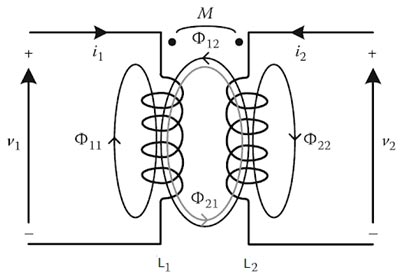
Consider two coils having self-inductances L1 and L2 placed very close to each other. Let the number of turns of the two coils be N1 and N2 respectively. Let coil-1 carries current I1 and coil- 2 carries current i2.
Due to current i1, the flux produced is Φ1 which links with both the coils. Then the mutual inductance between two coils can be written as
[latex display=”true”]M = \dfrac{{{{\rm{N}}_1}{\Phi _{21}}}}{{{i_1}}}[/latex]
Where Φ21 is the part of the flux Φ1 linking with the coil 2. Hence we can write Φ21 = K1Φ1
Where K1 = coefficient of coupling of coil-1
[latex display=”true”]M = \dfrac{{{{\rm{N}}_1}({K_1}{\Phi _1})}}{{{i_1}}}—–1[/latex]
Similarly due to current i2, the flux produced is Φ2 which links with both the coils. Then me mutual inductance between two coils can be written as
[latex display=”true”]M = \dfrac{{{{\rm{N}}_2}{\Phi _{12}}}}{{{i_2}}}[/latex]
Where Φ12 is the part of the flux Φ2 linking with the coil 1. Hence we can write Φ12 = K2Φ2
[latex display=”true”]M = \frac{{{{\rm{N}}_2}({K_2}{\Phi _2})}}{{{i_2}}} – – – – – 2[/latex]
Multiplying Equation 1 & 2
[latex]\begin{array}{l}{M^2} = \dfrac{{{{\rm{N}}_1}({K_1}{\Phi _1})}}{{{i_1}}} \times \dfrac{{{{\rm{N}}_2}({K_2}{\Phi _2})}}{{{i_2}}}\\\\{M^2} = {K_1}{K_2}\left[ {\dfrac{{{{\rm{N}}_1}{\Phi _1}}}{{{i_1}}}} \right]\left[ {\dfrac{{{{\rm{N}}_2}{\Phi _2}}}{{{i_2}}}} \right]\\\\{\text{Where }}\left[ {\dfrac{{{{\rm{N}}_1}{\Phi _1}}}{{{i_1}}}} \right] = {\text{ Self inductance of coil 1 = }}{{\rm{L}}_1}\\\\\left[ {\dfrac{{{{\rm{N}}_2}{\Phi _2}}}{{{i_2}}}} \right] = {\text{ Self inductance of coil 2 = }}{{\rm{L}}_2}\\\\\therefore {M^2} = {K_1}{K_2}{{\rm{L}}_1}{{\rm{L}}_2}\\\\M = \sqrt {{K_1}{K_2}} .\sqrt {{{\rm{L}}_1}{{\rm{L}}_2}} \\\\{\text{Let K = }}{K_1}{K_2}\\\\M = K\sqrt {{{\rm{L}}_1}{{\rm{L}}_2}} \\\\{\text{Where K = Coefficient of coupling}}\\\\\therefore K = \dfrac{M}{{\sqrt {{{\rm{L}}_1}{{\rm{L}}_2}} }}\end{array}[/latex]
The coefficient of coupling gives an idea about the magnetic coupling between the two coils. So when the entire flux in one coil links with the other, the coupling coefficient is maximum. The maximum value of K is unity. Thus when k = 1, the coupled coils are called tightly or perfectly coupled coils.
When the mutual inductance between the two coils is maximum with k = 1. The maximum value of the mutual inductance is given by
M = √L1L2
When the two coils are at a greater distance in space, the value of k is very small. Then the two coils are called loosely coupled coils.
Note:- k is the non-negative fraction and has the maximum value at unity.
(ii) Self-Inductance
When the current in a coil increases or decreases, there is a change in the magnetic flux linking the coil. Hence an e.m.f. is induced in the coil (called self-induced E.M.F ) which opposes the change of current in the coil (Lenz’s law). This phenomenon is called self-induction.
The phenomenon of production of opposing e.m.f in a coil when the current through the coil changes is called self-induction. The self-induced e.m.f. opposes the change of current in the coil
Thus when the current in the coil is increasing the self- induced e.m.f is produced in the coil in such a direction so as to oppose the increase in current i.e. the self-induced e.m.f. acts in a direction opposite to that of the applied voltage V.
When the current in the coil is decreasing the self-induced e.m.f. is produced in the coil in such a direction so as to oppose the decrease in current i.e., self-induced e.m.f. acts in the direction of applied voltage V.
COEFFICIENT OF SELF INDUCTION (or SELF INDUCTANCE)
Self-inductance is measured in terms of coefficient of self-inductance L. It obeys faraday’s law of electromagnetic induction like any other induced EMF.
Thus self-inductance of a coil opposes the change of current (increase or decrease) through the coil. This opposition occurs because a changing current produces self-induced e.m.f. (es) which opposes the change of current. That is why self-inductance of a coil is called electrical inertia of the coil.
Expressions for self-inductance (L).
We now find two equivalent expressions for self-inductance L of a coil (or circuit).
(i) Consider a coil of N turns carrying a current I. Suppose the magnetic flux linked with each turn of the coil due to this current is Φ. Then the flux linkages with the coil will be NΦ.
It is found that:
NΦ ∝ I
or NΦ = Ll
where L is a constant of proportionality and is called coefficient of self-induction or self-inductance of the coil.
[latex]L = – \dfrac{{N\Phi }}{I}[/latex]
Hence the coefficient of self-inductance of a coil is equal to the number of flux linkage with the coil when unit current is flowing through the coil.
(ii) If changing the current through a coil of N turns produced self-induced E.M.F (es) then
[latex]\begin{array}{l}{e_s} = – N\dfrac{{d\Phi }}{{dt}} = – \dfrac{d}{{dt}}(N\Phi )\\\\{\text{As we Know that N}}\Phi {\text{ = LI}}\\\\{e_s} = – \dfrac{d}{{dt}}(LI) = – L\dfrac{d}{{dt}}\\\\{e_s} = – L\dfrac{d}{{dt}}\end{array}[/latex]
where dl/dt is the rate of change of current in the coil in Weber/second.The negative sign shows that self-induced e.m.f. (es) is always in such a direction so as to oppose the change of current in the coil.
[latex]L = – \dfrac{{{e_s}}}{{dI/dt}}[/latex]
If dI/dt = 1, then L = -es
Hence coefficient of self-inductance of a coil is numerically equal to the self-inductance EMF in the coil when the rate of change of the current in the coil is unity.
S.I unit of Self-Inductance
The S.I unit of self-Inductance is Henry.
[latex]\begin{array}{l}{e_s} = – L\dfrac{{dI}}{{dt}}\\\\{\text{If }}\dfrac{{{\rm{dI}}}}{{dt}} = 1A/s\\\\e = 1V\\\\L = 1H\end{array}[/latex]
A coil or a circuit has self-inductance of 1 Henry if current changing at the rate of 1 ampere per second through the coil induced EMF of 1V in it.
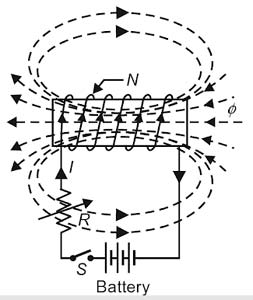
Factors affecting the self-inductance
Factors affecting the self-inductance of a conductor system are:
- The number of turns: More turns gives higher self-inductance;
- The way the turns are arranged: A short thick coil will have higher self-inductance than a long, thin one
The presence of a magnetic circuit: If the coil is wound on an iron core, the same current will set up a greater magnetic flux and the self-inductance will be higher.
(iii).
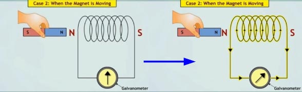
Electromagnetic Induction:-
The principle of electromagnetic induction state that if an electrical conductor is exposed to a changing magnetic field (magnetic lines of flux, a voltage will be induced into that conductor.
Electromagnetic induction was first discovered by Michael Faraday, who made his discovery public in 1831.It was discovered independently by Joseph Henry in 1832.
Faraday gave two important laws known as Faraday Law of electromagnetic induction:
First Law: When the magnetic flux through a circuit is changing, an induced electromotive force (E.M.F) is set up whose magnitude at any instant is equal to the negative rate of change of magnetic flux. This is also called Neumann’s Law.
If Φ is the magnetic flux linked with the circuit at any instant and e, the induced e.mf. then,
[latex display=”true”]e = – \dfrac{{d\Phi }}{{dt}}[/latex]
The minus sign is an indication of the direction of the induced e.m.f and this equation is called Faraday’s Law of induction.
If the circuit is a tightly wound coil of N turns, then the induced e.m.f. is
[latex display=”true”]e = – N\dfrac{{d\Phi }}{{dt}}[/latex]
Where
e = induced voltage in volts
N = Number of turns in wire
Φ = Magnetic flux in Weber
t = time in seconds
Factor Needed for Electromagnetic Induction to occur
- An electric conductor
- Magnetic Line of flux
- Relative motion between electric conductor and magnetic line of flux
Relative Motion.
The term “relative motion” means that the electrical conductor or, the magnetic lines of flux, or both that move to create the relative motion. A stationary magnetic field may have a moving electrical conductor pass through it to induce a voltage into the conductor, or a stationary electrical conductor may have a moving magnetic field pass through it. If both are moving it is still considered to be relative motion, unless they are both moving in the same direction and rate in relation to each other.
Factor affecting the Electromagnetic induction
The magnitude of the induced voltage from electromagnetic induction can be controlled, and is proportional to the following three factors:
- The number of turns of wire
- Magnetic flux density
- The speed of cutting action.
Number of Turns of Wire: If the electrical conductor is wound into a coil, each wire turn of the coil will have a voltage induced into it, and the induced voltages from all of the turns of wire will be of the same polarity. The effect of all the wire turns of the coil will be like a series circuit of many batteries connected together in the same polarity, and each will add together to equal their total sum. The more turns of wire in a coil, the greater the induced voltage will be.
Magnetic Flux Density: The strength of the magnetic field is measured by the number of magnetic lines of flux there are in a given cross-sectional area; the more lines of magnetic flux, the stronger the magnetic field. The greater the magnetic flux density, the more lines of magnetic flux are available to cut through the electrical conductor(s) for a given speed of cutting action, and the greater will be the induced voltage.
The speed of Cutting Action: Relative motion between the electrical conductor and the magnetic lines of flux is the speed of cutting action; the faster the magnetic lines of flux cut through the electrical conductor, the greater will be the induced voltage.
(iv) Time constant:
A general conceptual definition of a time constant can be given as follows:
A time constant is a measure of the time it takes to observe significant changes in a given process.
In physics and engineering, the time constant, usually denoted by the Greek letter τ (tau), is the parameter characterizing the response to a step input of a first-order, linear time-invariant (LTI) system. The time constant is the main characteristic unit of a first-order LTI system.
In an electric circuit consisting of a capacitor (C) and the resistor (R). We can define the time constant τc for the circuit:
τc = RC
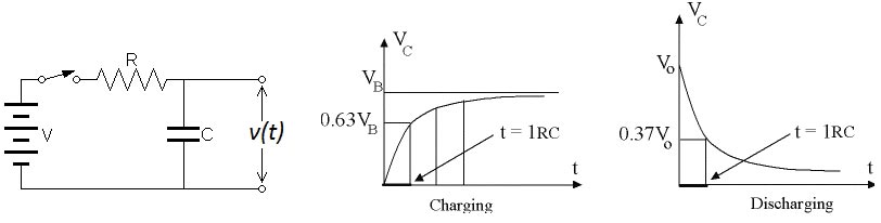
When capacitor is charging
The time constant of the R-C series circuit is defined as the time required by the capacitor voltage to rise from zero to 0.632 of its final steady state value during charging. i.e
Vc = 0.632V
When capacitor is discharging
When the capacitor discharge the time constant can be defined as the time required for charging current of the capacitor to fall to 0.368 of its initial maximum value, starting from its maximum value.
i = –0.368(V/R)amps
The negative sign indicates that the direction of discharge current is the reverse of that charging current.
From the above discussion, the time constant of an R-C series circuit can be defined as the time in seconds during which the voltage across the capacitor, starting from zero, would reach its final steady value if its rate of change was maintained constant at its initial value throughout the charging period.
Significance of Time Constant
The ‘time constant’ (I) of the circuit has following significance.
- The whole charging or discharging process can be considered to be completed in a time equal to 4 times the time constant and the current falls to insignificant value (theoretically the process takes infinite time).
- The charging current falls to 36.8% of its initial value in a time equal to time constant (τ) and to nearly 1.8% of initial value in, t = 4τ
- The capacitor charges to nearly 63.2% of its final value in, t = τ and nearly 98.2% of the final value in, t = 4τ provided it is initially uncharged.
- The capacitor discharges to nearly 36.8% of its initial value in, t = τ and nearly 1.8% of its initial value in, t = 4τ
- If the initial rate of rising voltage is maintained then the capacitor charges to its final value at a time = τ
Ques 2(c). A capacitor of 10 μF takes a current of 2A when an alternating voltage is applied across is 220 V, Calculate
(i) The frequency of the applied voltage
(ii) The resistance to be connected in series with the capacitor to reduce the current in the circuit to 1 A at the same frequency.
(i) Given
The capacitance of a capacitor C = 10μF = 10 × 10-6 F
Current I = 2 A
Voltage V = 220 V
Capacitive Reactance XC =?
Frequency f =?
The current, in amperes, in an ac circuit containing capacitance is determined using a form of Ohm’s law. i.e
I = V/XC
Hence the capacitive Reactance XC is
XC = V/I = 220/2 = 110Ω
Now the capacitive reactance of the circuit is given as
[latex]\begin{array}{l}{X_C} = \dfrac{1}{{2\pi fC}}\\\\\therefore f = \dfrac{1}{{2\pi C{X_C}}}\\\\ = \dfrac{1}{{2\pi \times 10 \times {{10}^{ – 6}} \times 110}}\\\\ = 144.68{\text{ }}Hz\end{array}[/latex]
(ii). When the resistance is connected in series with the capacitor

Impedance Z = V/I = 220/1 = 220Ω
Now in RC series circuit, the total Impedance is given by
[latex]\begin{array}{l}{Z^2} = ({R^2} + {X^2}_c)\\\\{220^2} = {R^2} + {110^2}\\\\R = \sqrt {{{220}^2} – {{110}^2}} \\\\R = \sqrt {48400 – 12100} \\\\R = 190.5\Omega \end{array}[/latex]
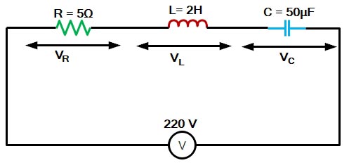
Ques 2(d). An RLC series circuit has R = 5Ω, C = 50μF and a variable inductance. The applied voltage is 220 V at 100 rad/sec. The inductance is varied till the voltage across resistance is maximum. Under this condition, find the
(i). Value of inductance
(ii) Q – Factor
(iii) Voltage across resistance, capacitance, and Inductance
Sol:- Given
Resistance R = 5Ω
Capacitance C = 50μF = 50 × 10-6 F
Voltage V = 220 V
Angular Frequency ωo = 100 rad/sec
Inductance L =?
Quality Factor Q =?
(i)The resonant frequency of the LC circuit is
[latex]\begin{array}{l}{\omega _o} = \dfrac{1}{{\sqrt {LC} }}\\\\100 = \dfrac{1}{{\sqrt {L \times 50 \times {{10}^{ – 6}}} }}\\\\{\left( {100} \right)^2} = \dfrac{1}{{L \times 50 \times {{10}^{ – 6}}}}\\\\L = \dfrac{1}{{500000 \times {{10}^{ – 6}}}}\\\\L = 2H\end{array}[/latex]
(ii) For an ideal series RLC circuit, the Q factor is
[latex]\begin{array}{l}Q = \dfrac{1}{R}\sqrt {\frac{L}{C}} = \dfrac{{{\omega _o}L}}{R}\\\\Q = \dfrac{{100 \times 2}}{5} = 40\end{array}[/latex]
(iii)
Current I = V/R = 220/5 = 44 A
Voltage across Resistance
VR = IR = 44 × 5 = 220 V
Voltage across Inductance
VL = QV = 40 × 220 = 8800 V
Voltage across capacitance
VC = QV = 40 × 220 = 8800 V