Ques.11. For the transfer function below, find the constraints on K1 and K2 such that the function will have only two poles on jω-axis?
[katex]T(s) = \dfrac{{{K_1}s + {K_2}}}{{{s_4} + {K_1}{s^3} + {s^2} + {K_2}s + 1}}[/katex]
K1 > K2
K1 = K2
K1 < K2
None of the above
Show Explanation
Answer.4. None of the above
Explanation
The characteristic equation of the system is:
s4 + K1 s3 + s2 + K2 s + 1 = 0
For the characteristic equation, we form the Routh’s array method as:
s4
1
1
1
s3
K1
K2
s2
[katex]\dfrac{{{K_1} – {K_2}}}{{{K_1}}}[/katex]
s1
[katex]T(s) = \dfrac{{{K_1}^2 – {K_1}{K_2} + {K_2}^2}}{{{K_2} – {K_1}}}[/katex]
s0
1
For the system having two imaginary poles, the required condition will be:
[katex]{K_1}^2 – {K_1}{K_2} + {K_2}^2[/katex]
Since the above equation has no real roots, therefore there is no relationship between K1 and K2 that will have just two jω-poles.
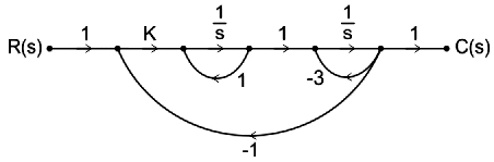
Ques.12. The signal flow graph of a system is given below. The system is stable for the value of K > ______
6
3
9
1
Show Explanation
Answer.2. 3
Explanation
The characteristic equation of the system is given by the signal flow graph (SFG) , i.e.
Δ = 1 – (L1 + L2 + L3 ) + L12
Where L1 , L2, and L3 are the individual loop gains and L12 is the gain of a pair of two-nontouching loops. For the given SFG of the system, we have
L1 = 1/s
L2 = −3/s
L2 = −k/s2
L12 = −3/s2
The determinant for the SFG can be calculated as:
[katex]\begin{array}{l} \Delta = 1 – \left( {\dfrac{1}{s} – \dfrac{3}{s} – \dfrac{K}{{{s^2}}}} \right) + \left( {\dfrac{{ – 3}}{{{s^2}}}} \right)\\ \\ = 1 + \dfrac{2}{s} + \dfrac{{K – 3}}{{{s^2}}}\\ \\ q\left( s \right) = 1 + \dfrac{2}{s} + \dfrac{{K – 3}}{{{s^2}}} = 0 \end{array}[/katex]
According to the Routh array characteristics Methods
Thus, the required condition for the stability of the system is: A block diagram is shown below. The transfer function for this system is
K – 3 > 0
Or K > 3
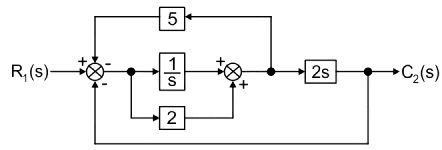
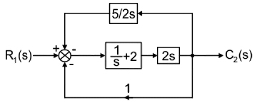
13. A block diagram is shown below. The transfer function for this system is
[katex]\dfrac{{2s\left( {2s + 1} \right)}}{{2{s^2} + 10s + 5}}[/katex]
[katex]\dfrac{{2s\left( {2s + 1} \right)}}{{2{s^2} + 23s + 5}}[/katex]
[katex]\dfrac{{2s\left( {2s + 1} \right)}}{{4{s^2} + 3s + 5}}[/katex]
[katex]\dfrac{{2s\left( {2s + 1} \right)}}{{4{s^2} + 13s + 5}}[/katex]
Show Explanation
Answer.4. [katex]\dfrac{{2s\left( {2s + 1} \right)}}{{4{s^2} + 13s + 5}}[/katex]
Explanation:-
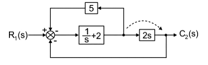
The given block diagram is shown below:
Here, the two branches having gains 1/s and 2 are in parallel hence they will be added.
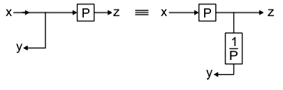
Now, we change the take-off position of the block of 2s
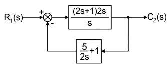
Again, both feedback branches are parallel, therefore adding the gain we get:
Thus, using feedback formula, we obtain the overall transfer function as:
[katex]\begin{array}{l} T\left( s \right) = \dfrac{{G\left( s \right)}}{{1 + G\left( s \right)H\left( s \right)}}\\ \\ = \dfrac{{\dfrac{{\left( {2s + 1} \right)2s}}{s}}}{{1 + \dfrac{{\left( {2s + 1} \right)2s}}{s} \times \dfrac{{\left( {5 + 2s} \right)}}{{2s}}}}\\ \\ = \dfrac{{2s\left( {2s + 1} \right)}}{{s + \left( {2s + 1} \right)\left( {5 + 2s} \right)}}\\ \\ = \dfrac{{2s\left( {2s + 1} \right)}}{{4{s^2} + 13s + 5}} \end{array}[/katex]
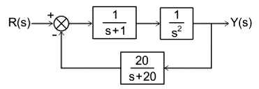
14. Which of the following options is correct for the system shown below?
3rd order and unstable
4th order and unstable
3rd order and stable
4th order and stable
Show Explanation
Answer.2. 4th order and unstable
Explanation:-
From the block diagram,
[katex]\begin{array}{l} G\left( s \right) = \frac{1}{{{s^2}\left( {s + 1} \right)}}\\ \\ H\left( s \right) = \frac{{20}}{{\left( {s + 20} \right)}} \end{array}[/katex]
As the given feedback is negative, the transfer function of the closed-loop system is
[katex]\begin{array}{l} \frac{{Y\left( s \right)}}{{R\left( s \right)}} = \frac{{G\left( s \right)}}{{1 + G\left( s \right)H\left( s \right)}}\\ \\ = \frac{{\frac{1}{{{s^2}\left( {s + 1} \right)}}}}{{1 + \frac{1}{{{s^2}\left( {s + 1} \right)}}\frac{{20}}{{\left( {s + 20} \right)}}}}\\ \\ = \frac{{s + 20}}{{{s^2}\left( {s + 1} \right)\left( {s + 20} \right) + 20}}\\ \\ = \frac{{s + 20}}{{{s^4} + 21{s^3} + 20{s^2} + 20}} \end{array}[/katex]
In the above transfer function denominatior has highest value of 4. Therefore, the order of the system is 4.
The coefficient of ‘s’ term is zero in the characteristic equation (denominator of above transfer function). Therefore, the system is unstable.
15. Transfer function of a compensator is given by
Gc(s) = (s + a)/(s + b)
GC (s) is a lead compensator if
a =−3, b = −1
a = 3, b = 2
a = 3, b = 1
a = 1, b = 2
Show Explanation
Answer.4. a = 1, b = 2
Explanation
General form of lead compensator is given as
Gc(s) = (s + z)/(s + p)
Here
z = 1/T, P = 1/αT
For lead compensator
α = Z/P < 1
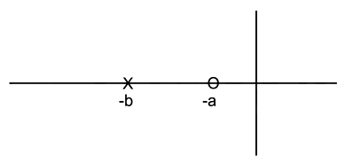
The pole-zero location of lead compensator in s-plane is given as
For phase lead compensator, a < b
Option (4) is correct i.e a = 1, b = 2
15. A system transfer function is excited by sin(ωt). The steady-state output of the system is zero at
[katex]G\left( s \right) = \frac{{\left( {{s^2} + 9} \right)\left( {s + 2} \right)}}{{\left( {s + 1} \right)\left( {s + 3} \right)\left( {s + 4} \right)}}[/katex]
ω = 8 rad/sec
ω = 4 rad/sec
ω = 3 rad/sec
ω = 1 rad/sec
Show Explanation
Answer.3. ω = 3 rad/sec
sin ω t → G ( s ) → Y ( s ) = | G ( s ) | ⋅ sin ( ω t + ∠ G ( s ) )
The output will be zero when
|G(s)| = 0
Put s = jω
[katex]\left| {\frac{{\left( { – {\omega ^2} + 9} \right)\left( {j\omega + 2} \right)}}{{\left( {j\omega + 1} \right)\left( {j\omega + 3} \right)\left( {j\omega + 4} \right)}}} \right| = 0[/katex]
For the value ω = 3 , |G(jω)| = 0
16. A closed-loop system has the characteristic equation given by s3 + Ks2 + (K + 2)s + 3 = 0. For this system to be stable, which one of the following conditions should be satisfied?
K > 1
0.2 < K < 1
0 < K < 0.2
K < 1
Show Explanation
Answer.1. K > 1
Explanation
Given that characteristic equation is,
s3 + Ks2 + (K + 2)s + 3 = 0
s3
1
(K + 2)
s2
K
3
s1
[K(K + 2) − 3]/K
0
s0
3
For stable system,
K > 0, K (K + 2) – 3 > 0
⇒ K > 0, K2 + 2K – 3 > 0
⇒ K > 0, (K + 3) (K – 1) > 0
⇒ K > 0, K > -3, K > 1
⇒ K > 1
17. Match the transfer functions of the second-order systems with the nature of the systems given below.
Transfer Function
Nature of Sytem
A:- [katex]\frac{{15}}{{{s^2} + 5s + 15}}[/katex]
1:- Underdamped
B:- [katex]\frac{{25}}{{{s^2} + 10s + 25}}[/katex]
2:- Critically damped
C:- [katex]\frac{{35}}{{{s^2} + 18s + 45}}[/katex]
3:- Overdamped
A ⇒ 1, B ⇒ 2, C ⇒ 3
A ⇒ 2, B ⇒ 1, C ⇒ 3
A ⇒ 3, B ⇒ 2, C ⇒ 1
A ⇒ 3, B ⇒ 1, C ⇒ 2
Show Explanation
Answer.1. A ⇒ 1, B ⇒ 2, C ⇒ 3
Explanation:-
The second-order system is given by the equation
[katex]\frac{{\omega _n^2}}{{{s^2} + 2\xi {\omega _n}s + \omega _n^2}}[/katex]
If ξ = 1, then the system is critically damped.
If ξ < 1, then the system is underdamped.
If ξ > 1, then the system is order damped.
[katex]A = \frac{{15}}{{{s^2} + 5s + 15}}[/katex]
By comparing the second order transfer function,
ωn 2 = 15 ⇒ ωn = √15
[katex]2\xi {\omega _n} = 5 \Rightarrow \xi = \frac{5}{{2\sqrt {15} }} < 1[/katex]
Hence it is an underdamped equation
[katex]B=\frac{{25}}{{{s^2} + 10s + 25}}[/katex]
ωn 2 = 25 ⇒ ωn = 5
2 ξ ωn = 10 ⇒ ξ = 1
So, it si critically damped system.
[katex]C = \frac{{35}}{{{s^2} + 18s + 45}}[/katex]
ωn 2 = 35 ⇒ ωn = √45
[katex]2\xi {\omega _n} = 18 \Rightarrow \xi = \frac{9}{{\sqrt {35} }} > 1[/katex]
So, it is overdamped system.
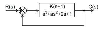
18. The positive values of ‘K’ and ‘a’ so that the system shown in the figure below oscillates at a frequency of 2 rad/sec respectively are
3, 0.49
05, 0.5
2, 2
2, 0.75
Show Explanation
Answer.4. 2, 0.75
Explanation:-
Characteristic equation:
s3 + as2 + (2 + k) s + (k + 1) = 0
s3
1
(K + 2)
s2
a
(K + 1)
s1
[katex]\frac{{a\left( {k + 2} \right) – \left( {k + 1} \right)}}{a}[/katex]
0
s0
k + 1
[katex]\frac{{a\left( {k + 2} \right) – \left( {k + 1} \right)}}{a} = 0[/katex]
a = (K + 1)/(K + 2)—— (1)
For oscillator
as2 + k + 1 = 0
s2 = ω2 = -4
-4a + k + 1 = 0 – – – – (2)
Solving equation (1) & (2) we get
a = 0.75 & k = 2
19. The unit step response of an under-damped second-order system has a steady-state value of -2. Which one of the following transfer functions has these properties?
(1) [katex]\frac{{ – 3.24}}{{{s^2} + 2.59s + 1.12}}[/katex]
(2) [katex]\frac{{ – 1.58}}{{{s^2} – 2.59s + 1.12}}[/katex]
(3) [katex]\frac{{ – 3.82}}{{{s^2} – 1.91s + 1.91}}[/katex]
(4) [katex]\frac{{ – 3.82}}{{{s^2} + 1.91s + 1.91}}[/katex]
Show Explanation
Answer. [katex]\frac{{ – 1.58}}{{{s^2} – 2.59s + 1.12}}[/katex]
Explanation-
[katex]T\left( s \right) = \frac{{k\:\omega _n^2}}{{{s^2} + 2\xi {\omega _n}s + \omega _n^2}}[/katex]
Under damped system ξ < 1
[katex]\xi = \frac{{1.91}}{{2\sqrt {1.91} }} = 0.69[/katex]
Only option 2 is correct
20. A lead compensating network
Improves response time
Stabilizes the system
Increases resonant frequency
All of the above
Show Explanation
Answer.4. All of the above
Explanation:-
Lead compensator increases relative stability by increasing phase margin.
For a LEAD COMPENSATOR, bandwidth INCREASES as zero is added to the transfer function, ie. s in the numerator, as an effect, the damping factor increases thereby increasing the bandwidth. [bandwidth = 2x(damping factor)]
Due to phase-lead controller (compensator) amplification at higher frequencies, it increases the bandwidth of the compensated system. The phase-lead controllers are used to improve the gain, resonant frequency, and phase stability margins and to increase the system bandwidth (decrease the system response rise time).