31. The signal flow graph of a system is shown below. The transfer function of the system is
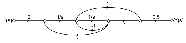
- (S + 1)/(S − 1)
- (S + 1)/(S2 + S + 1)
- (S − 1)/(S + 1)
- (S − 1)/(S2 + S + 1)
Answer.2. (S + 1)/(S2 + S + 1)
Explanation:-
Applying Masson’s gain formula
- Capacitance
- Inductance
- Elastance
- Resistance
Answer.3. Elastance
Explanation:-
Force Voltage Analogy
| Translational | Electrical |
| Force (F) | Voltage (v) |
| Mass (M) | Inductance (L) |
| Damper (D) | Resistance ( R) |
| Spring (K) | Elastance (1/C) |
| Velocity (u) | Current (i) |
| Displacement (x) | Charge (q) |
Hence from the Force voltage analogy, the spring is reciprocal of Capacitance i.e Elastance.
33. Static error coefficients are used as a measure of the effectiveness of closed-loop systems for specified ________ input signal.
- Acceleration
- Position
- Velocity
- All of the above
Answer.4. All of the above
Explanation:-
Steady-State Error: For a step excitation, the difference between the desired output and the final value of any system is termed as the steady-state error of the system.
[katex]E(s) = \dfrac{{R(s)}}{{1 + G(s)H(s)}}[/katex]
Position, Velocity and Acceleration Error Constant
| S.No | Constant | Equation | Steady-state error |
| 1 | Position error constant (Kp) | [katex]{K_P} = \mathop {Lt}\limits_{s \to 0} G(s)H(s)[/katex] | [katex]{e_{ss}} = \frac{A}{{1 + {K_P}}}[/katex] |
| 2 | Velocity error constant (Kv) | [katex]{K_v} = \mathop {Lt}\limits_{s \to 0} sG(s)H(s)[/katex] | [katex]{e_{ss}} = \frac{A}{{{K_v}}}[/katex] |
| 3 | Acceleration error constant (Ka) | [katex]{K_a} = \mathop {Lt}\limits_{s \to 0} {s^2}G(s)H(s)[/katex] | [katex]{e_{ss}} = \frac{A}{{{K_a}}}[/katex] |
Advantage of Coefficient of error methods
- This method is applicable only to the three standard input signals and cannot give error coefficients for other input signals.
- Mathematical response of error, i.e., 0 or cannot give an exact value of error.
- This method can provide the important time variation of error.
- This method can be used for stable systems
34. The type 1 system has ______ at the origin.
- 3 Poles
- 0 Poles
- 1 pole
- Infinite Poles
Answer.3. 1 pole
Explanation:-
The type of system is significant to predict the nature of this error.
• A system having no pole at the origin is referred to as a Type-0 system.
• Thus, Type-1, refers to one pole at the origin and so on.
35. The position and velocity errors of a type-2 system are
- Zero, constant
- Zero, Zero
- Constant, Constant
- Constant, Infinity
Answer.1. Zero, constant
Explanation:-
It also follows that a type 0 system would have a non-zero finite position error and infinite velocity and acceleration errors.
A type I system would have a non-zero finite velocity error, a zero position error, and an infinite acceleration error.
A type 2 system would have a non-zero finite acceleration error and zero velocity and position errors. Thus, knowing the system type number, only one error needs to be determined and the others are either zero or infinite.
| System | Step Input r(t) = 1 |
Ramp Input r(t) = t |
Acceleration Input r(t) = 1/2 t2 |
| Type 0 | 1/1 + K | ∞ | ∞ |
| Type 1 | 0 | 1/K | ∞ |
| Type 2 | 0 | 0 | 1/K |
The terms “position error”, “velocity error”, “acceleration error” mean steady-state deviations in the output position. A finite velocity error implies that after transients have died out, the input and output move at the same velocity but have a finite position difference.
The error coefficient Kp, Kv, and Ka describe the ability of a system to reduce or eliminate steady-state error. It is desirable to increase the error coefficients while maintaining the transient response within an acceptable range. From the above Table, it can be seen that
- A type 0 system gives an error for all three types of inputs.
- It also follows that a type 0 system would have a non-zero finite position error and infinite velocity and acceleration errors.
- A type I system would have a non-zero finite velocity error, a zero position error, and an infinite acceleration error.
- A type 2 system would have a non-zero finite acceleration error and zero velocity and position errors. Thus, knowing the system type number, only one error needs to be determined and the others are either zero or infinite.
A type 2 system gives an error due to one type of input only, which is finite. So a type 2 system is better than a type 0 system or a type I system from the steady-state error point of view. Higher types of systems are better from the steady-state error point of view but are less stable.
Thus type 0 and type 1 systems are capable of following a parabolic input. For a type 2 system, the error is finite, but for type 3 or higher systems, the error is zero. Again as we increase the type numbers, the error goes on reducing.
36. Velocity error constant of a system is measured when the input to the system is unit _______ function.
- Parabolic
- Ramp
- Impulse
- Step
Answer.2. Ramp
Explanation:-
Static Velocity Error Coefficient (Kv)
Static velocity error coefficient is associated with ess for a unit ramp input. When the input to the system is unit ramp function then only velocity error is finite but the error due to other inputs are not defined.
The steady-state actuating error of the system with a unit ramp input (unit velocity input) is given by
[katex]{K_v} = \mathop {Lt}\limits_{s \to 0} sG(s)H(s)[/katex]
For ramp input, the steady-state error for the type 0 system is infinite. Hence, a type 0 system is not capable of following ramp input. The static velocity error for the type 1 system is finite. But static velocity error for the type 2 systems or higher systems is zero. So type 2 or higher systems are capable of following a ramp input very accurately. As we move from type 0 to type 2 or higher systems, the static velocity error goes on decreasing. But with an increase in the type number, the number of poles on the JW-axis also goes on increasing, which will make the system response more oscillatory. Hence, we have to make a compromise between stability and accuracy.
37. In the case of a type-1 system steady-state acceleration is
- Unity
- Infinity
- Zero
- None of the above
Answer.3. Zero
Explanation:-
Static acceleration error coefficient is associated with ess for a unit parabolic input. The steady-state actuating error of the system with unit-parabolic input (acceleration) is given by
[katex]{K_a} = \mathop {Lt}\limits_{s \to 0} {s^2}G(s)H(s)[/katex]
For type 1 system steady state error is zero.
37. If a step function is applied to the input of a system and the output remains below a certain level for all the time, the system is
- Stable
- Unstable
- Always unstable
- Marginally stable
Answer.4. Marginally stable
Explanation:-
A linear time-invariant system is said to be stable if it satisfies the following conditions:
- Even after excitation by a bounded input, the output must be bounded
- In the absence of input, the output must be zero irrespective of initial conditions.
Absolute stability: The stability of the system with respect to variation of parameters is known as absolute stability. It said to be absolutely stable when it is stable for all values of the parameters.
Relative stability: It measures the degree of stability and it is a quantitive measure of how fast the system transients die out in a system. Conditional stability: The stability of the system with respect to its parameter variation is known as conditional stability.
Marginally Stable System
A system is Marginally Stable if the natural response neither decays nor grows but remains constant or oscillates within a bound
• The open-loop control system is marginally stable if any two poles of the open-loop transfer function are present on the imaginary axis.
• Similarly, the closed-loop control system is marginally stable if any two poles of the closed-loop transfer function is present on the imaginary axis.
Step Input
The step function has a fixed amplitude for all-time arguments. Thus, shifting it or delaying it does not change the sampled values. We conclude that the modified z-transform of a sampled step is the same as its z-transform, times z−1 for all values of the time advance mT—that is, 1/(1 — z−1)
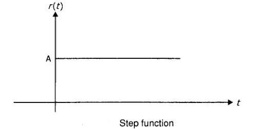
Since a step function neither decays nor grows but remains constant hence it is marginally stable.
38. Which of the following is the best method for determining the stability and transient response?
- Root locus
- Bode plot
- Nyquist plot
- None of the above
Answer.1. Root Locus
Explanation:-
Root Locus for Determining Stability
- The root locus method for determining the stability of a system is literally a plot of all the possible locations on the complex plane for the roots of the characteristic equation of that system if the gain is allowed to vary from zero to infinity.
- If the location of all the roots of the closed-loop system is in the negative part of the complex plane, the system is stable
- If any of the roots of the closed-loop system are positive for certain values of gain, the corresponding root locus plot will lie in the positive part of the complex plane.
- The root locus method was first described by W. R. Evans, who has done a great deal to demonstrate its effectiveness. The root locus method lends itself to a greater understanding of the transient response performance of the system, rather than its frequency response, as does the Nyquist criterion. It has the ability to demonstrate directly the effect on the closed-loop response of the changes in the open-loop system gain from zero to infinity.
- Although changes in the time constants or complex roots of the open-loop are not directly indicated, effects of changes in them are generally fairly evident from the plot with the original values.
- From this method it is possible to determine the absolute decrement rate of the exponential factors from the negative real part, of the root, and also the decay time expressed in terms of its ratio to the frequency of oscillation from the ratio of the real portion of the root to its distance from the origin.
39. Phase margin of a system is used to specify which of the following?
- Frequency response
- Absolute stability
- Relative stability
- Time response
Answer.3. Relative stability
Explanation:-
Relative stability:- By relative stability, we mean how close the system is to instability, and we can improve the stability of the system. The degree or extent of the system is called relative stability.
Phase Margin: If φ is the phase angle of a system at unity gain, the phase margin is given by (180 + φ). The frequency (ω) at which gain is unity is known as gain crossover frequency. The increment in the system angle that causes the system to be unstable is indicated by the phase margin. It is a measure of relative stability.
40. Addition of zeros in transfer function causes which of the following?
- Lead-compensation
- Lag-compensation
- Lead-lag compensation
- None of the above
Answer.2. Lag-compensation
Explanation:-
Effect of addition of zeros: Addition zeros to the loop transfer function produces a phase lead that tends to stabilize the closed-loop control system. The root loci of a two-pole configuration have been shown in Fig. If a zero is added at s = −b as shown in Fig (b), the resultant root loci will bend towards the left. The stability margin is therefore increased.
The addition of Zeros to a given function gives
[katex]\begin{array}{l} G(s)H(s) = \frac{K}{{s(s + a)}}\\ \\ G(s)H(s) = \frac{{K(s + b)}}{{s(s + a)}};b > a \end{array}[/katex]
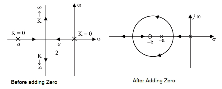
Adding zero to the function of G(s)H(s) has the effect of moving the RL(Root Locus) towards the left half.
Result of Addition of Zero
- All branches of RL now lie completely left half of the s-plane, so K can be adjusted to any positive value without causing instability.
- By complete RL are now bent toward to LHS of s-plane from jω-axis.
- By suitable adjustment of zero (compensating) along the negative axis, the steady-state error is within the limit.
- The addition of zero in transfer function causes lag compensation of s-plane. A similar effect will result if a pair of complex-conjugate zero is added to the function.
The effects of addition of zeros are as follows:
- There is a change in the shape of the root locus and its shifts towards the left of the s-plane.
- The stability of the system is enhanced.
- Range of K increases.
- Setting time speeds up.
Effects and limitations of a lag compensator:
The lag compensator has the following effects and limitations:
- Since the lag compensator allows high gain at low frequencies, it is basically a low pass filter. Therefore, it improves the steady-state performance.
- In lag compensation, the attenuation characteristics is used for the compensation, whereas the phase lag characteristics is of no use in compensation.
- Since the attenuation due to a lag compensator shifts the gain crossover frequency to a lower frequency point, the bandwidth of the system is reduced. Hence a slower response occurs. Therefore, rise time and settling time are usually longer and hence the transient response lasts for a longer time.
- The system is very sensitive to parameter variation.
- Since a lag compensator approximately acts as a proportional plus integral controller, it thus tends to make a system less stable.